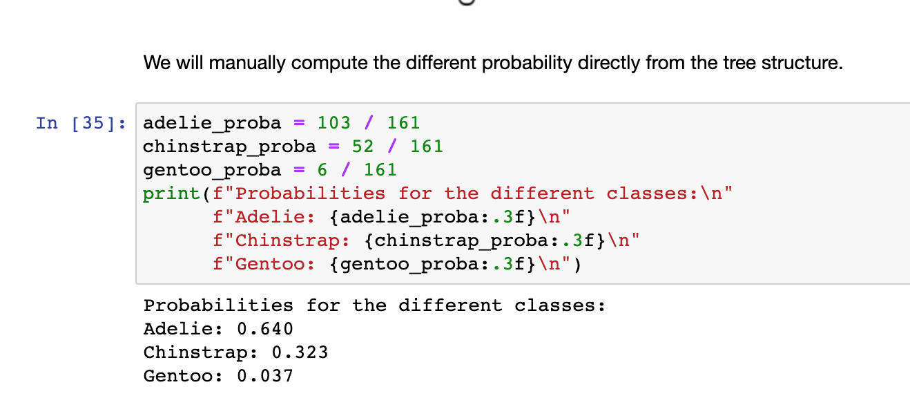
Q2) When computing probabilities manually, we use values in the right leaf (sub-sample of 161). Presumably, we could have used the values in the left leaf too (sub-sample of 95), no?
Our target contains 3 classes. So we have a multiclass problem.
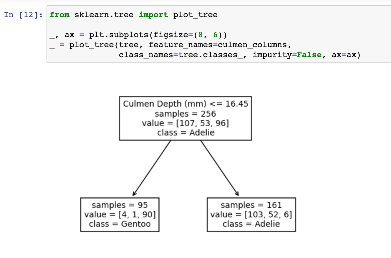
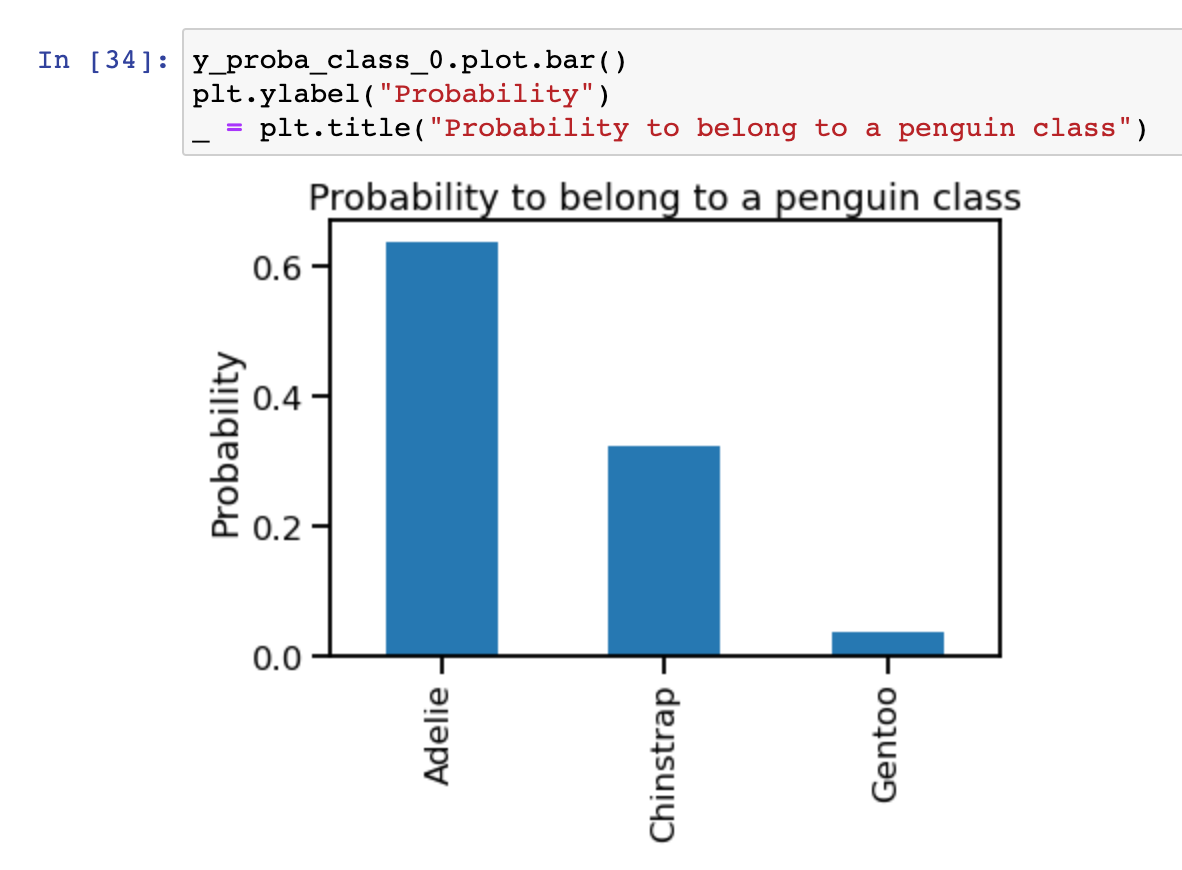
When building a tree with a depth of 1 (thus a single split), we can only split the data into 2 partitions and thus define two leaves. The class predicted at each leaf will be the most represented class. Thus on the left side, the Gentoo has 90 samples far ahead of Adelie and Chinstrap. For the right leaf, the story is a bit more complicated. We have many samples from Adelie and Chinstrap, 103 and 52, respectively. Thus we will predict Adelie because it is the majority class. However, in terms of probability, we know that you have 2 chances over 3 to be Adelie and 1 chance over 3 to still be Chinstrap. Hard predictions do not convey this message because we completely discard that Chinstrap samples were present at this leaf.
Computing the probability of the left leaf will give you information if the Culmen Depth is lower than 16.45 mm while the right leaf will give information if you are above this threshold. Then, we can compute probability statistics for both leaves indeed.
With a deeper tree, the only difference is that you will partition the feature space first and then for a specific area of the feature space compute statistics as the probabilities based on the training set.
The probabilities will be meaningful for the hyperrectangle defined by the different decision taken across the tree. In the next exercise, you will get a better intuition on the effect of increasing the depth, and thus increasing the number of rectangles and therefore defining a local probability rule for this specific rectangle.