
How and what do we infer from the box plot of coefficient variation? If the IQR is more, does it mean that particular variable explains enough variance in the data?
If the box for a coefficient is large, it means it varies a lot with the randomization of the data. So for instance, with a coefficient that would vary between 0 and 100, 0 would mean that the feature will not be considered to predict the target while with 100, it will have an influence (to be more precise regarding the impact of this feature, we would also need to look at the other coefficient values).
So usually, if one tries to get inside regarding what a linear model does, he/she will look at these coefficients. If you have a large variation of a coefficient, it is then impossible to conclude regarding the importance of this feature: sometimes it is important and sometimes not just by changing slightly the data. On the contrary, if the coefficients are very stable, you can draw better intuitions.
I can give a concrete example by taking some discussion from the following example: Common pitfalls in interpretation of coefficients of linear models — scikit-learn 1.0.dev0 documentation
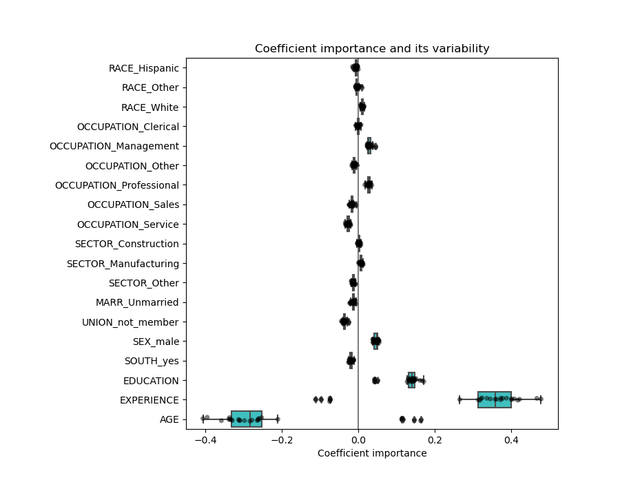
You can see that AGE and EXPERIENCE have really large boxes. Indeed, this effect is sometimes linked with correlated variables: on a dataset, the experience was chosen to be important and thus age became neglected by the model while on another set, the opposite happened.
If you decide to remove one of the two variables will get the following:
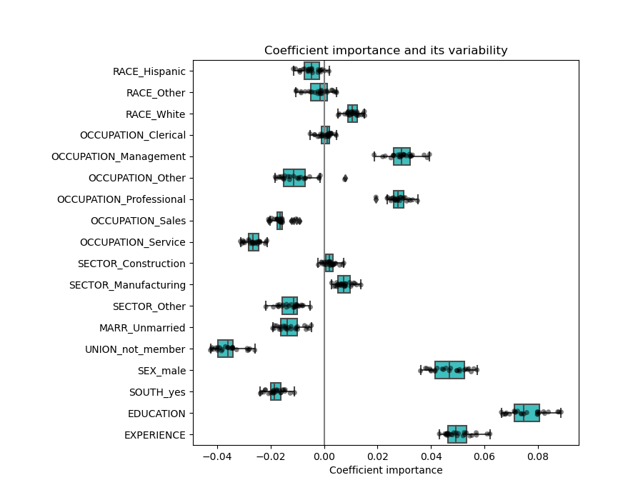
Now, EXPERIENCE is stable and does not vary a lot anymore and you can draw some insights.
1 Like
@glemaitre58
Just to clarify more, after removing the Age variable, other variables that previously is located towards 0 coefficient are now having large coefficient. In this case, should we test out whether it is better off to remove Experience variable and maintain Age variable to check whether other variables will stay at large coefficient or small coefficient?
Back to the lecture’s boxplot, the first boxplot is using only PolynomialFeatures while the second boxplot is using PolynomialFeatures and Ridge.
I am still a bit confuse on how to determine which one is better as the first boxplot having move variables is near to 0 while the second one having more variables having bigger and away from 0 coefficient. Can you highlight this point?
In the course, what you should understand is why the values are all close to zero with some large coefficients or why they are all kinda better distributed. The reason is that without scaling the features, the range is really different for each feature and thus are the coefficients. Linear models expect to have all features with a close range of values.
What you observe in the boxplot in the course, is a consequence to properly scaling the feature as expected by linear modelling.
ok, thanks for the guidance.
When the coefficient is closed to zero, it means that the regularization is effective in controlling the model overfitting issue.
When I compare the 3 graphs (A.=PolynomialFeature, B=A + Ridge and C=B+StandardScaler), my finding is:
A is mostly coefficient close to zero
B is still close to zero but coefficient is more spread out
C more coefficient is spread out but in small scale and slightly away from zero
Therefore, C meets the objective of able to control overfitting to some extend and coefficient spread is not wide, meet linear equation objective. Does my understanding is correct?
I think so
1 Like